15 Excel Data Analysis Tips for Non Nerds from Shopper Intelligence
I confess I am not an expert
I use Excel all the time, but I confess I am not an expert and don’t have the time to figure out better ways to do the things I do regularly (and the things I am guessing many commercial analysts need to do). So, I asked our tech team here at Shopper Intelligence what features of Excel they find particularly helpful for day to day data analysis. I chose 15 that I don’t currently use but were most relevant.
I thought I’d share them with you!
– Roger Jackson, CEO Shopper Intelligence

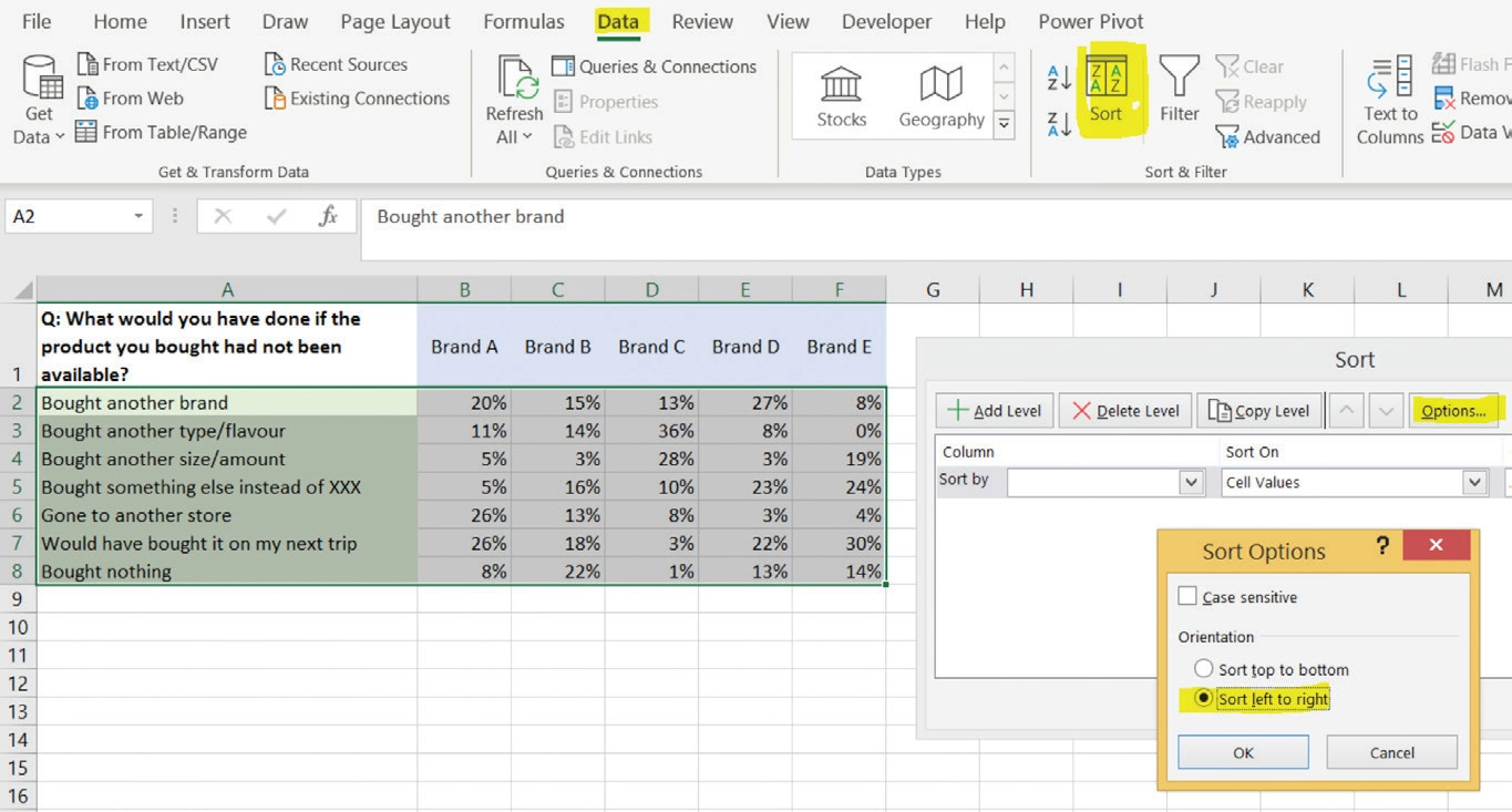
1. Horizontal sorting (left to right)
Do you use vertical sorting? It’s a daily standard, right? But what do you do when you want to sort your table horizontally? Many of us copy and transpose the table and then sort it vertically. I know I do. But, hey, there is an easier way…
This has helped me to compare items in a table in both ways, for example looking at the top mentions for a brand, and also simultaneously ranking the brands on a certain attribute. Especially with a long list of hundreds of categories and brands, as in our shopper database.
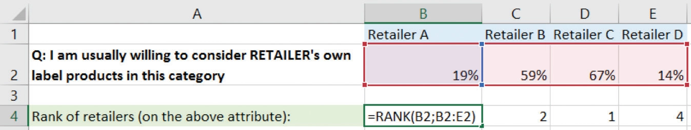
2. Rank function
This one is dead simple, and can save a lot of repeated manual sorting.
Maybe I seem to be obsessed with ranking things – it may come from spending too much time with our shopper database comparing hundreds of categories. Or watching too much Formula-1? Anyway….
Let’s say you want to rank 5 different brands based on their scores on the Price attribute. Of course you can do it with the regular sort button, but when you have several image items, you may not want to sort the brands repeatedly. Instead, you want to have a neat table with the ranks visible on all the attributes at the same time.
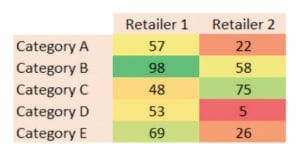
3. Conditional formatting – pre-set styles
Conditional formatting is a useful tool when you have data in a table format (especially a big table) and you want to see the key information at a glance: showing the high and the low spots visually. It’s also easy to use.
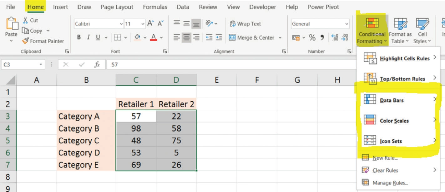
You just need to select the cells that you want to format, and then go directly from
Home > Conditional Formatting and select one of the pre-defined styles (or set up your own rule).
Many of us just try one style and stick with it. Even though the different styles can serve different purposes. A few examples:
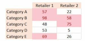
a) Colour scale: Values are colored from bright red (lowest value in table) to dark green (highest value in table) like a heatmap. It’s easy to see which cells are the darkest green and brightest red, and you can compare any values at a glance. Use this if you want to compare the RELATIVE values of all the cells at once. It’s also good when you want to look for a few OUTLIERS in a big table (e.g. find the cell with value 1 out of all the cells with value 0). They will clearly pop out in your eyes.
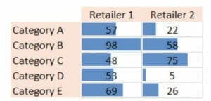
b) Data bars: Cells are filled up with a selected color, based on their values. Basically like a hor- izontal bar chart. Use this if you are also interest- ed in the ABSOLUTE values as well. In the Colour scale view, the lowest value will always be red, so you will know which is the smallest value, but not necessarily know how small it is (until you look at the number). In the Data bar view you also see how big or small that value is in absolute terms, not only compared to other cells.
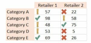
c) Icon Sets: Little icons are added to each cell, marking whether they are higher or lower than the average or on par. It is a simplified view, because rather than having a million different shades, you only have 3 (or 4 or 5) different icons. Use it when you just want to see a SIMPLE CLASSIFICATION (is the value small, medium or high?). Also, there are many different icon sets to choose from.
d) Top/Bottom Rules: The Top 5 (or 10, or as many as you define) values are simply highlighted. This is again helpful when you only need to see the top values rather than comparing all the values in the table.
And this is where to find it:
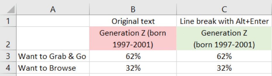
4. Line break within a cell [Alt+Enter]
Often you want to write some text in an Excel cell (e.g. a title), and you want to start the next word in a new line within the same cell (e.g. some explanation).
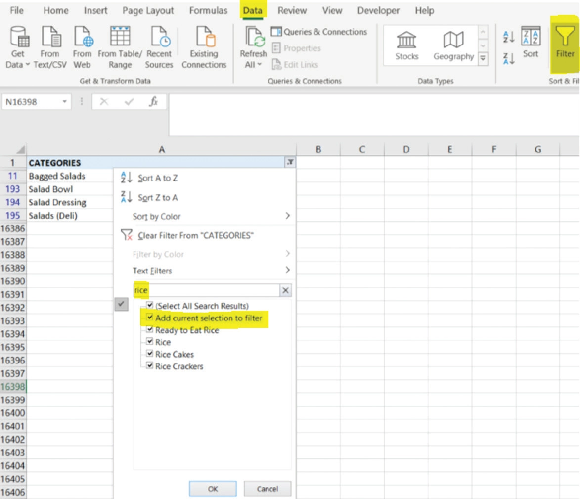
5. Keep the selection of multiple searches in a filter
Say you have a long list of items and you want to see only the items that contain either “Sal- ad” or “Rice” (or both). You add a filter (Data > Filter) and type your search words. How to do this properly? You can’t type both words, and if you type Salad, then select the items, then type Rice, then you’ll lose your Salad selections.
Instead, what you need to do is, do it in 2 steps and in the second step, tick “Add current selection to filter” at the beginning of the list.
That will do the trick. You will have a list with Salad and Rice. Bon appetit!
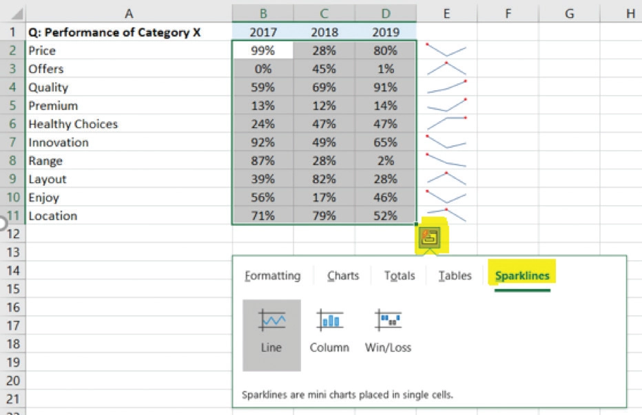
6. Sparklines (=mini charts in single cells)
Sparklines are super useful. They are basically a set of mini charts each placed in a single Excel cell, and they allow you to take a snapshot of the trend for different rows at the same time, without the effort (and space in your workbook) of creating an actual detailed chart with different colors and legends.
For example, you want to look at the trend of each attribute over a period of time (in the case of our data they could be for a specific category). You just want to know whether their trend is going up or down. Perhaps you want to know if for several markets or channels at the same time. You can incorporate many of these in your dashboard or KPI report.
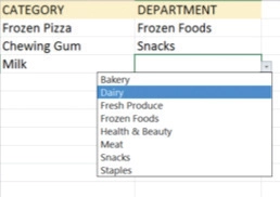
7. Create a drop-down list
They have multiple usages. Most often you want to use this because you want to control what can be written in a cell (i.e. only one of the pre-defined answer options), or you want to make it easier to fill in the cell (e.g. avoid mistyping or having several versions of an item).
It is helpful and easy to do. In the example let’s say you have a list of categories in the first col- umn, and in the second column, next to each category you want to add the department where it belongs. You can do it in 2 steps:
Step 1. Make a list of the possible departments that you want to allow to be selected. Put it somewhere far on the sheet or even on a separate sheet (here it’s in cells G2-G9), because you don’t need it to be near the data.
Step 2. Select the cell where you want the drop-down menu to appear (here it is in B2, the De- partment of the first category Frozen Pizza). Go to Data > Data Validation > Data Validation > Settings. In “Allow” select “List” and in “Source” select your department list (cells G2-G9). Click OK.
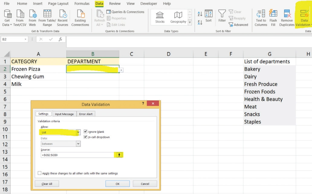
You are ready. When you click on the cell, the drop-down list appears and allows you to make your selection from the pre-defined options. Moreover, you can copy this cell and the drop-down list will be copied to the new cells, too.
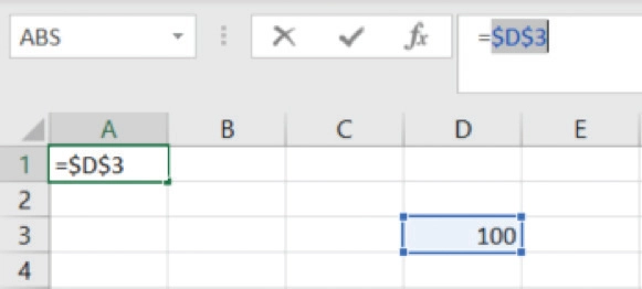
8. Quickly fix a cell reference in an Excel formula using the key F4
Here’s a simple, but very cool time saving trick. When you use a function or formula in Excel, and you reference a cell (e.g. cell D3), you need to be careful when you copy it to other cells. If you don’t fix the columns or the rows with a dollar sign ($), then the formula remains relative, and it adjusts automatically (so if you copy it to a cell to the right and one cell down, it will reference cell E4 instead of D3).
Depending on what you want to fix (rows, columns or both), you need to add a dollar sign be- fore the column identified (e.g. $D) or before the row identifier (e.g. D$3) or both (e.g. $D$3). Honestly, it can be annoying and prone to error to do this multiple times.
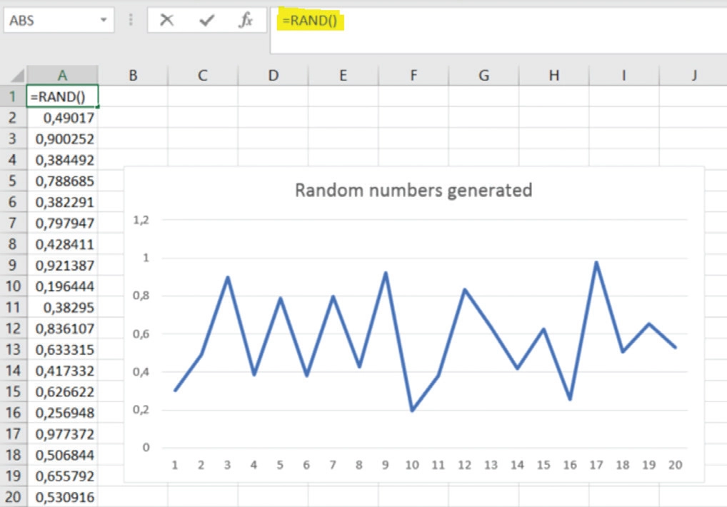
9. Random number generator
I am always creating dummy charts (e.g. if I am figuring out a new graphic for our data). To create a dummy chart or table, instead of typing numbers randomly for minutes, it is easier to do it with a function.
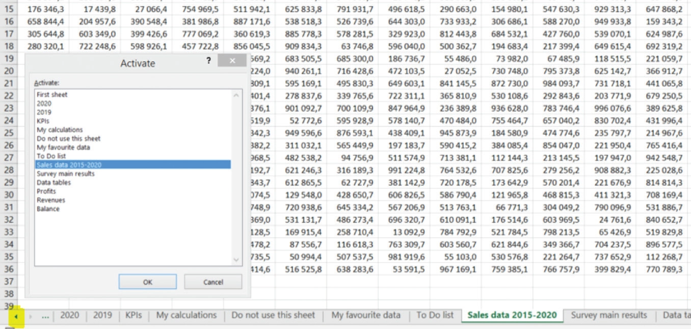
10. Easily find a sheet in a huge Excel file
Some Excel files can have tens of sheets and it can be difficult and time consuming to nav- igate between them, because you can’t see all the sheet names at once so you scroll from left to right and then back..
Smart people colour the sheet tabs, to highlight the more important ones (click right on the tab and go to Tab colour). What is less often used is that you can actually have the sheets listed and select the one you want to go to. Once the sheet list is in a vertical format, it’s already easier to see them.
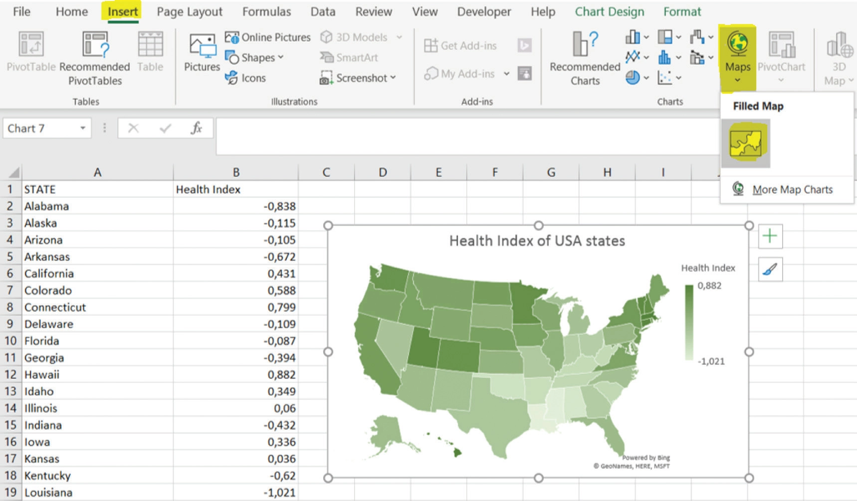
11. Show data on a map easily in Excel
It can be tough to get excited about Excel, but honestly, this is really cool. I surely thought you would need a separate tool for this – a software, an app or a website. But it’s a built-in feature in Excel (2016 onwards).
Below is the map of the USA states coloured based on the Health Index of each state (data source: United Health Foundation). It works with any map of the world.
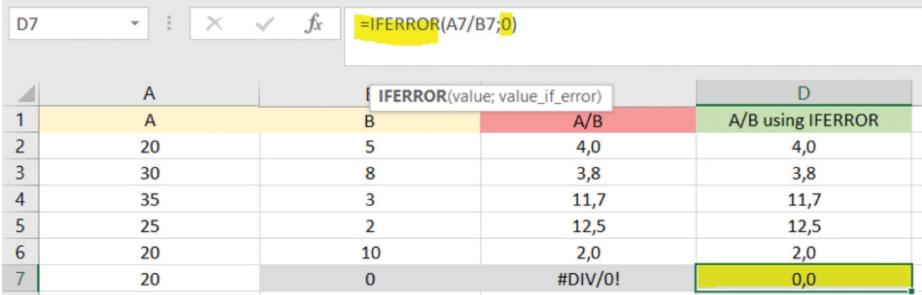
12. Manage cell errors with the IFERROR function
If you use basic Excel functions you have certainly experienced that sometimes the result is something that looks like an error (e.g. #VALUE!, #NAME?, #DIV/0!, and so on). Sometimes you want to deal with it (because your formula is wrong and you need to correct it), and sometimes you want to ignore it (e.g. because it’s caused by an empty cell somewhere).
In this second case (i.e. making Excel ignore the error), the IFERROR function is a big help.
Example: in cells C7 and in D7 we used the same formula: calculate A7/B7. In C7 this gives us an error (#DIV/0!, error of division by zero), but in cell D7 we added IFERROR and “0” as the outcome. So we asked Excel to put the value “0” if the A7/B7 calculation resulted in an error. So the result is 0.
This is helpful when you later want to reference this cell.
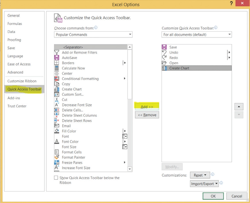
13. Customize your Excel shortcut menu
There are functions in Excel that we each use regularly. We know where to find them in the menu, but sometimes it takes 3 or 4 clicks to get there. Wouldn’t it be nice to reach them directly?
There is a shortcut menu in Excel. It’s the one you see on the very top of your screen, with the Save icon, the Undo and the Redo buttons by default.
That shortcut menu is customizable. You can add any of your favorite functionalities and you’ll always have them available within a click. Do you like to filter or sort your data very often? Do you freeze panes on a regular basis? Or simply do you want the Open File button to be available with a single click? Put these icons in the shortcut and your work in Excel be- comes quicker and more efficient.
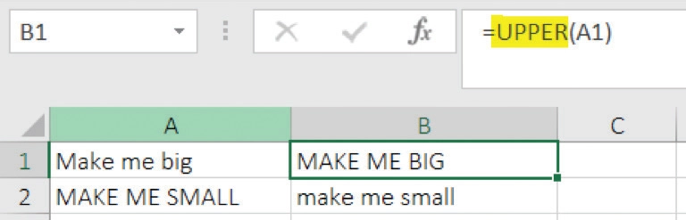
14. Change text to upper case
In Word you change the case of a text (lowercase/uppercase) with a button. In Excel there is no such button (why, Microsoft, why?), but it’s still relatively easy to change the case of a text.
To change to all uppercases, use the UPPER() function. To change to lowercases, use the
LOWER() function.
There are other exciting functions with texts in Excel. (OK I know the word exciting might not be exactly the one I’d use ordinarily but, heh, times change! ) I would honestly encourage you to explore them.
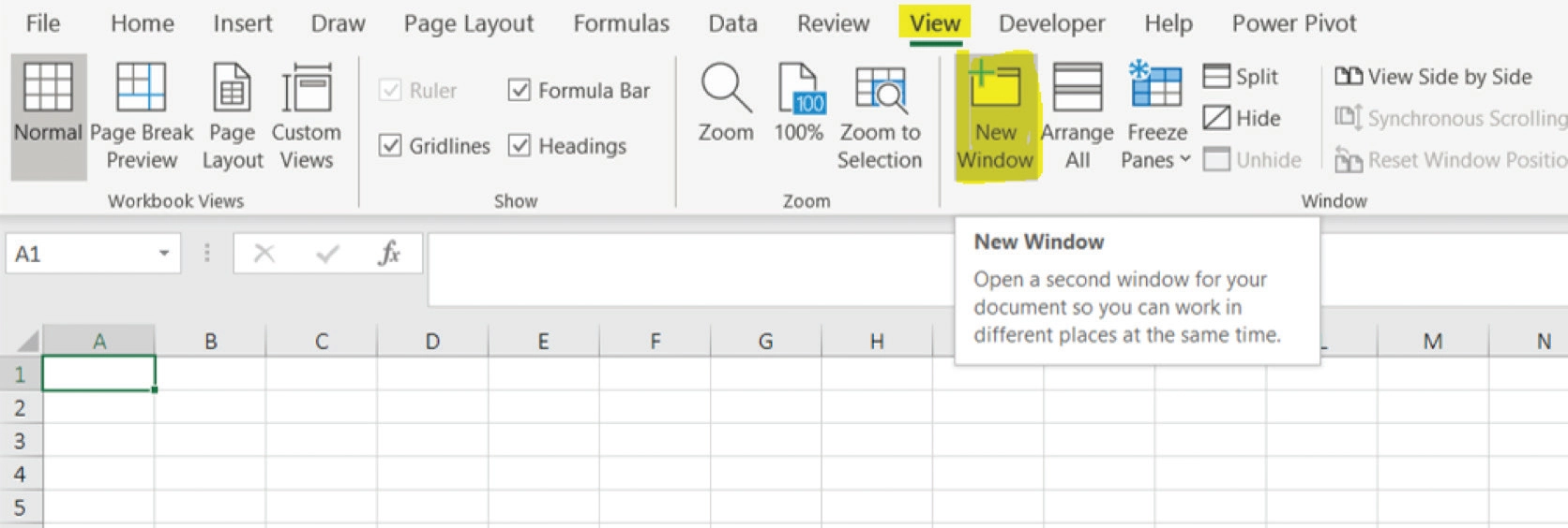
15. Open the same file twice simultaneously
This is especially useful when you work on two screens (e.g. a laptop and a monitor), and you can use two parts of the same spreadsheet at the same time. But it’s also useful when you just don’t want to switch between sheets of a file all the time.